Which Is The Graph Of Linear Inequality 6x 2y 10
Next Genwave
Mar 06, 2025 · 5 min read
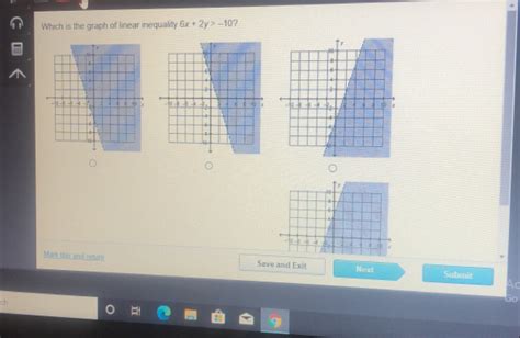
Table of Contents
Which is the Graph of Linear Inequality 6x + 2y ≤ 10? A Comprehensive Guide
Understanding linear inequalities and their graphical representations is crucial in various fields, from mathematics and economics to computer science and engineering. This comprehensive guide delves into the process of graphing the linear inequality 6x + 2y ≤ 10, explaining each step in detail and offering insights into related concepts. We'll cover everything from converting the inequality to a more manageable form to understanding shading and boundary lines.
Understanding Linear Inequalities
A linear inequality is a mathematical statement that compares two expressions using inequality symbols such as < (less than), > (greater than), ≤ (less than or equal to), and ≥ (greater than or equal to). Unlike linear equations, which have a single solution, linear inequalities have a range of solutions. These solutions can be represented graphically as a region on a coordinate plane.
The general form of a linear inequality in two variables is:
Ax + By ≤ C (or using other inequality symbols)
where A, B, and C are constants, and x and y are variables.
Steps to Graph 6x + 2y ≤ 10
Let's break down the process of graphing the linear inequality 6x + 2y ≤ 10 step-by-step:
Step 1: Convert to Slope-Intercept Form (y = mx + b)
While not strictly necessary, converting the inequality to slope-intercept form makes graphing easier. The slope-intercept form clearly shows the slope (m) and the y-intercept (b) of the boundary line.
To convert 6x + 2y ≤ 10 to slope-intercept form, we need to isolate y:
- Subtract 6x from both sides: 2y ≤ -6x + 10
- Divide both sides by 2: y ≤ -3x + 5
Now we have the inequality in the form y ≤ mx + b, where m = -3 (the slope) and b = 5 (the y-intercept).
Step 2: Graph the Boundary Line
The boundary line represents the equation y = -3x + 5. This is a straight line. We can graph this line using two methods:
-
Using the y-intercept and slope: The y-intercept is 5, so the line passes through the point (0, 5). The slope is -3, meaning for every 1 unit increase in x, y decreases by 3 units. We can use this information to find another point on the line, such as (1, 2). Connect these two points to draw the line.
-
Using two points: Choose any two convenient values for x, substitute them into the equation y = -3x + 5, and calculate the corresponding y values. Plot these two points and draw a line connecting them. For example:
- If x = 0, y = 5 (Point: (0, 5))
- If x = 1, y = 2 (Point: (1, 2))
Crucial Note: Because our original inequality is "less than or equal to" (≤), the boundary line should be a solid line. If the inequality were strictly "less than" (<), the boundary line would be a dashed line, indicating that the points on the line itself are not part of the solution set.
Step 3: Determine the Shaded Region
The inequality y ≤ -3x + 5 means that we are looking for all points (x, y) where the y-coordinate is less than or equal to -3x + 5. This defines a region below the line.
To determine which side of the line to shade, choose a test point that is not on the line. The origin (0, 0) is often a convenient choice, unless the line passes through the origin.
Let's test the point (0, 0):
y ≤ -3x + 5 0 ≤ -3(0) + 5 0 ≤ 5
This inequality is true. Since the test point (0, 0) satisfies the inequality, we shade the region that includes the origin – the region below the line.
Step 4: The Complete Graph
The complete graph of the linear inequality 6x + 2y ≤ 10 consists of the solid line y = -3x + 5 and the shaded region below it. Every point in the shaded region, including the points on the solid line, represents a solution to the inequality.
Interpreting the Graph
The shaded region represents the solution set of the inequality. Any point (x, y) within this region will satisfy the inequality 6x + 2y ≤ 10. Points outside the shaded region will not satisfy the inequality.
For example, the point (1, 1) is within the shaded region:
6(1) + 2(1) = 8 ≤ 10 (True)
However, the point (2, 5) is outside the shaded region:
6(2) + 2(5) = 22 > 10 (False)
Advanced Concepts and Applications
Understanding linear inequalities extends beyond simple graphing. Here are some advanced concepts and real-world applications:
Systems of Linear Inequalities
Often, we deal with multiple linear inequalities simultaneously. This forms a system of linear inequalities. Graphing a system involves graphing each inequality individually and then identifying the region where all inequalities are satisfied – the feasible region. This is commonly used in linear programming to find optimal solutions under constraints.
Bounded and Unbounded Regions
The solution set of a linear inequality (or a system) can be bounded (enclosed within a finite area) or unbounded (extending infinitely). The inequality 6x + 2y ≤ 10, for example, has an unbounded solution set because the shaded region extends infinitely downwards.
Linear Programming
Linear programming is a mathematical method used to optimize a linear objective function subject to linear constraints (inequalities). The graphical method of linear programming involves identifying the feasible region defined by the constraints and then finding the corner points of this region to determine the optimal solution. This has applications in resource allocation, production planning, and many other optimization problems.
Applications in Real-World Scenarios
Linear inequalities find applications in various real-world scenarios:
- Budgeting: Representing constraints on spending within a budget.
- Production planning: Determining the number of products to manufacture given resource limitations.
- Scheduling: Allocating time efficiently among various tasks.
- Resource allocation: Distributing resources optimally across different projects or departments.
- Game theory: Defining strategy spaces and constraints in game models.
Conclusion
Graphing linear inequalities, like 6x + 2y ≤ 10, is a fundamental skill with wide-ranging applications. By understanding the steps involved—converting to slope-intercept form, graphing the boundary line, choosing a test point to determine shading, and interpreting the shaded region—you can effectively visualize and interpret the solution set of such inequalities. Mastering this skill opens doors to more advanced concepts like systems of linear inequalities and the powerful techniques of linear programming, enabling you to solve complex optimization problems in various fields. Remember that practice is key! Work through several examples, varying the inequalities and their symbols, to solidify your understanding. The more you practice, the more confident you'll become in graphing and interpreting linear inequalities.
Latest Posts
Latest Posts
-
C 5 F 32 9 Solve For F
Mar 06, 2025
-
5 6 Divided By 3 5
Mar 06, 2025
-
6 25 Rounded To The Nearest Tenth
Mar 06, 2025
-
What Is The Square Root Of 625
Mar 06, 2025
-
What Is 6 To The Power Of 2
Mar 06, 2025
Related Post
Thank you for visiting our website which covers about Which Is The Graph Of Linear Inequality 6x 2y 10 . We hope the information provided has been useful to you. Feel free to contact us if you have any questions or need further assistance. See you next time and don't miss to bookmark.
