Y 2x 1 Y 2x 3
Next Genwave
Mar 09, 2025 · 6 min read
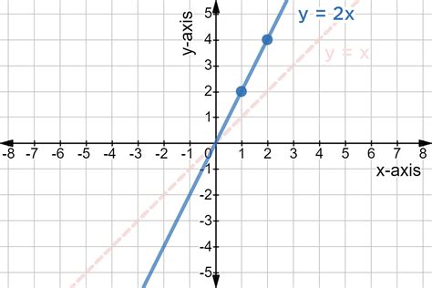
Table of Contents
Exploring the Mathematical Relationship: y = 2x + 1 and y = 2x + 3
The equations y = 2x + 1 and y = 2x + 3, while seemingly simple, offer a rich ground for exploring fundamental concepts in algebra and linear equations. Understanding their similarities and differences provides valuable insight into graphing, solving systems of equations, and interpreting the meaning of slope and y-intercept. This article delves deep into these equations, examining their individual properties and then comparing them to highlight key mathematical principles.
Understanding Linear Equations: The Basics
Before we dive into the specifics of y = 2x + 1 and y = 2x + 3, let's establish a foundational understanding of linear equations. A linear equation is an algebraic equation that represents a straight line when graphed on a coordinate plane. It's typically written in the slope-intercept form:
y = mx + b
where:
- y represents the dependent variable (the output)
- x represents the independent variable (the input)
- m represents the slope of the line (the rate of change of y with respect to x)
- b represents the y-intercept (the point where the line crosses the y-axis, where x = 0)
This form makes it easy to visualize and analyze the line's characteristics.
Analyzing y = 2x + 1
Let's examine the first equation, y = 2x + 1. By comparing it to the slope-intercept form, we can identify its key features:
-
Slope (m) = 2: This indicates that for every one-unit increase in x, y increases by two units. The line is positive sloping, meaning it rises from left to right.
-
Y-intercept (b) = 1: This means the line intersects the y-axis at the point (0, 1).
Graphing y = 2x + 1: To graph this equation, we can start by plotting the y-intercept (0, 1). Then, using the slope, we can find another point. Since the slope is 2 (or 2/1), we can move one unit to the right and two units up from the y-intercept, giving us the point (1, 3). Connecting these two points creates the line representing y = 2x + 1. You can continue this process to plot more points and ensure accuracy.
Analyzing y = 2x + 3
Now let's analyze the second equation, y = 2x + 3. Again, comparing it to the slope-intercept form reveals:
-
Slope (m) = 2: Identical to the first equation, the slope is 2. This means the line also rises two units for every one-unit increase in x.
-
Y-intercept (b) = 3: The line intersects the y-axis at the point (0, 3).
Graphing y = 2x + 3: Similar to the previous equation, we start by plotting the y-intercept (0, 3). Using the slope of 2, we can move one unit to the right and two units up from the y-intercept, leading us to the point (1, 5). Connecting these points gives us the line representing y = 2x + 3.
Comparing y = 2x + 1 and y = 2x + 3: Parallel Lines
The most striking observation when comparing these two equations is their parallelism. Both equations have the same slope (m = 2), which is the defining characteristic of parallel lines. Parallel lines never intersect; they maintain a constant distance from each other. This parallelism visually demonstrates that the lines represent different but related relationships.
Solving Systems of Equations: No Solution
Because the lines are parallel, there is no solution to the system of equations formed by y = 2x + 1 and y = 2x + 3. There is no point (x, y) that satisfies both equations simultaneously. Attempting to solve this system algebraically (e.g., using substitution or elimination) would result in a contradiction, confirming the absence of a solution.
Interpreting the Difference: The Constant Term's Significance
The difference between the two equations lies solely in their y-intercepts. The equation y = 2x + 3 has a y-intercept that is two units higher than the y-intercept of y = 2x + 1. This constant term (b) represents a vertical shift in the graph. Essentially, the line y = 2x + 3 is a vertical translation of the line y = 2x + 1, shifted upwards by two units. This concept is crucial in understanding transformations of functions.
Applications and Real-World Examples
While these equations may seem abstract, they have real-world applications. Consider these scenarios:
-
Linear Growth: Imagine two different investments, both growing at the same rate (slope = 2), but starting with different initial amounts (y-intercepts). One investment (y = 2x + 1) begins with a smaller initial value, while the other (y = 2x + 3) starts with a higher initial value. Both investments grow at the same rate, represented by the identical slopes, but their overall values differ due to the initial investment amounts.
-
Cost Models: Suppose two companies offer similar services but have different fixed costs (y-intercepts) and the same variable cost per unit (slope = 2). The equations would represent the total cost for each company as a function of the number of units produced. The difference in fixed costs would lead to different total costs for the same production level.
-
Temperature Conversion: Though not directly represented by these exact equations, the concept of parallel lines with different y-intercepts is relevant in temperature conversions. Celsius and Fahrenheit scales are linearly related but have different scales (y-intercepts) and rates of change (slopes).
Advanced Concepts and Extensions
The exploration of y = 2x + 1 and y = 2x + 3 can be extended to more advanced concepts:
-
Systems of Inequalities: Instead of equalities, we could consider inequalities (e.g., y > 2x + 1 and y < 2x + 3). Solving these would involve finding the regions on the coordinate plane satisfying both inequalities.
-
Linear Programming: These equations can be integrated into linear programming problems, which involve optimizing objective functions subject to linear constraints.
-
Vector Representation: The equations can be represented using vectors, providing a geometric perspective on the lines and their relationship.
Conclusion: A Foundation for Further Learning
The seemingly simple equations y = 2x + 1 and y = 2x + 3 offer a robust foundation for understanding fundamental concepts in algebra and linear equations. By analyzing their individual properties, comparing them, and considering their applications, we gain a deeper appreciation for the power and versatility of linear relationships. This analysis serves as a springboard for exploring more complex mathematical concepts and real-world applications. The parallelism of the lines highlights the significance of slope and y-intercept, emphasizing how small changes in the constant term can lead to significant differences in the overall relationship. The exploration of these equations showcases the beauty and practicality of mathematical principles in understanding and modeling various phenomena. This detailed analysis equips readers with a strong understanding of linear equations and prepares them for tackling more intricate mathematical challenges.
Latest Posts
Latest Posts
-
X 2 Y 2 9 Graph
Mar 09, 2025
-
Cuanto Es El 3 Por Ciento De 1000
Mar 09, 2025
-
10 6 Rounded To The Nearest Tenth
Mar 09, 2025
-
Escribe Tu Problema Y Te Lo Resolvemos
Mar 09, 2025
-
200 96 Rounded To The Nearest Tenth
Mar 09, 2025
Related Post
Thank you for visiting our website which covers about Y 2x 1 Y 2x 3 . We hope the information provided has been useful to you. Feel free to contact us if you have any questions or need further assistance. See you next time and don't miss to bookmark.
